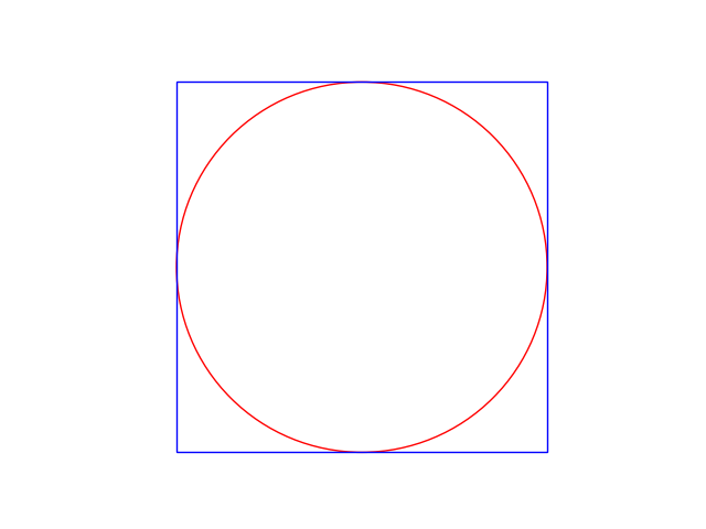
Figure 1: A circle within a square
This is almost every where the very first thing that is taught in MC. And I believe it is a good place to start. Here we want to see that MC simulation works by estimating the value of \(\pi\). In order to do that, we create a geometric situation in which we can somehow extract the number pi from it. One case is to create a circle with radius 1 which has an area of \(\pi\). So now as MC based methods are based on probability, we have to restate the problem in a probabilistic way. In order to do that, we can think of another shape that has a bigger area than the circle. we can take the encompassing square for more visual appeal! Now imagine a dart that is thrown randomly inside the square. The probability of the dart to land inside the circle is equal to the ratio of the area of circle to the square \(\frac{\pi}{4}\). So if we throw a lot of darts, and then count the number of darts that fell inside the circle to the total number of darts, we expact it to be equal to \(\frac{\pi}{4}\). So if we multiply the result by 4, we get an estimate for \(\pi\). Thats it!

Figure 1: A circle within a square
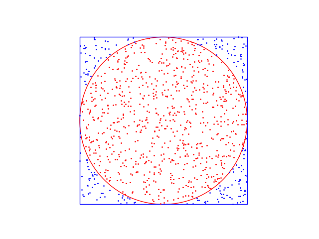
So now we have to simulate the dart throwing process. We can do that by generating random coordinates within the boundaries of the square
        no_of_points = 1_000_000
        x = np.random.uniform(-1, 1, no_of_points)
        y = np.random.uniform(-1, 1, no_of_points)
Then we can check if the coordinate is inside the circle or not. If it is, we count it as a hit.
        inside = x**2 + y**2 <= 1
        no_of_hits = np.sum(inside)
Then we calculate the ratio of the darts falling within the circle to the total number of darts. And multiply it by 4 to get an estimate for \(\pi\).
pi = 4 * no_of_hits / no_of_points

Figure 2: Darts Flying!
Here we have used 1,000,000 points and it gave an estimation of 3.144. Not bad!